
 I recently resurrected a Microsoft Excel spreadsheet I built to budget out 12 months to assess the likely impact of moving back to Australia – which included a combined 50% drop in salary and an increase in expenses. This was 2008 – but I now find myself doing something similar. My income has dropped (closer to 30%) and my living circumstances have changed significantly as well, thanks to COVID-19 – albeit, my life is a lot cheaper (if not leaner) now …
In my usual fashion of putting off an actual decision, I decided once again to SpreadSheet the frack out of the problem, and have decided to tidy it up and make it available for anyone else to use. Without further adieu I present … the Infinidim Budget Planning Spreadsheet. Hopefully this will be of use to anyone out there who might need to look at their reduced Income vs Outgo, or just generally want a simple tool to look at budget planning is a reasonably comprehensive, sophisticated way.
Infinidim Budget Planning Spreadsheet
The current version can be downloaded via the purple links just below this paragraph. I will keep an update of the version history here as I make any further changes to the sheet. Note – you will not be able to use this on a Mac (OSX) or in an iPad (IOS) because I had to write some visual basic code in the back of the spreadsheet to do some of the more complex calculations. That said – if you set it up in Windows/PC you can certainly open it on your Mac/iPad and it should display – it just won’t re-calculate. Remember (Virgin Crew) you have access to Excel through the Company portal and it will work there if you email it to yourself.
- Update 01-Jul-2020 : This update tidies up the sheet with some further bells and whistles, including some buttons to add/remove rows, and zoom the sheet to the appropriate size. See the training video for an update on the new features.
- 22-Apr-2020 : This initial release is a complete re-work of the previous development, separating the global Income and Expense parameters into separate sheets for clarity. I’ve also added the functionality to do a Weekly Analysis (16 weeks) as well as the previous Monthly Analysis (12 months). As before, you can establish your parameters to look at different scenarios – such as the world going back to normal in July vs not until the end of August (or later).
Training Videos
I have made a series of Training Videos for the spreadsheet on my YouTube Channel. No. it’s not that hard to use if you know Excel – but if not, watching me get it started and hearing me blather on about it should actually help. You can access the Infinidim Budget Planner playlist to work through the videos, or scroll down the very bottom of this article to watch them here. Don’t forget to increase the YouTube stream quality to maximum, otherwise you might not be able to make out the detail in the training video.
Overview
Basically this spreadsheet allows you to create a master list of all your sources of Income – as well as your Expense Items. When such items are cyclical (as so many of them tend to be) – the spreadsheet allows you to express them in this way, for example …
- 50% Salary; of $1000; paid Fortnightly; previously paid on 09.Apr.20; last planned payment on 18-Jun-20
- 100% Salary; of $2000; paid Fortnightly; next pay 02-Jul-20; continues after that without end.
- Health Insurance; $1500; paid quarterly; next due on 15.Aug.20
- Bank Mortgage; $1150; paid on the 1st of each month (Monthly); next due 01.May.20; continues until 01.May.2031
- Car – Petrol; $20; per Week on a Wednesday (Weekly).
- … etc
You can see that if you can (a) create a reasonably accurate forecast of your income and (b) a reasonably comprehensive list of most of your expenses – a spreadsheet can combine these together and look at any period. The next 12 months; and/or the 12 months after that; the next 16 weeks (2x56 day or 4×28 day rosters); the 16 weeks after a return to 100% salary. The level of accuracy comes from how accurately you track your bills. Which is not a bad place to start when budgeting.
Let’s get into it, shall we?
Note : Before the Training Videos, there is a short section on using Excel. This area doesn’t really teach you Excel, but it does go through a few of the basic manipulations such as adding rows, sizing columns, locking and unlocking the worksheet(s). If you really don’t know how to use Excel – watch the videos and then look through this section first.
The Income Sheet
This is probably the simplest sheet in the spreadsheet. Into here you enter any/all of your income streams. This could be as simple as your fortnightly salary; but also include Centrelink payments, rental income, forecast Etsy earnings, etc.
Note : There is some complexity to setting up the Income and (particularly) the Expenses sheets. While watching the training videos should get you through this – the best advice I can give is to complete one line in the Income (or Expenses) sheet – then go to the Planning tab, select in your newly created Income/Expense – and see how it maps out across the Months/Weeks. It should be pretty clear straight away if it is/is not working.
As always – The GREEN areas are designed for your input. The rest of the sheet is locked to ensure you don’t damage the structure/formulas.
Finally – while the instructions here start in the Income Sheet; then go onto the Expenses Sheet; and finally to the Planning sheet – my recommendation is that each time you add an Income or an Expense – go straight to a Planning Sheet and select in that new Income or Expense and see how it’s worked. This will verify your Ref Date / Regularity / Start-Stop Date settings, and allow you to tweak them
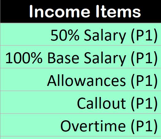 1. Income Item (name)s
This column is just the “name” of the Income item. Apart from allowing you to keep track of your income streams – this name is used in the Planning Windows to select income for analysis. Keep it short, clearly understandable, simple. You’ll be selecting them from a list in those sheets. Remember that you may want to create multiples for a single item – such as “House Insurance (Quarterly)” vs “House Insurance (Yearly)” – so make the names logical.
2. Allocation
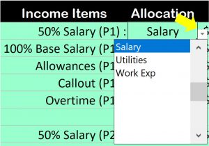
Presently this it not (really) in use – but I have plans to add graphs that will amalgamate and analyse income/expenses based on this Allocation tag. For example, in expenses if you add a “Cars” Allocation to all your car expenses (Petrol, Insurance, Registration, Maintenance, etc) then once I have it sorted you can group together all these costs into one “Cars” analysis. At least that’s the theory – does anyone actually want that?
Note that Allocation can be selected from a drop-down list. Click on the little down arrow next to the cell and choose from the list (working this way tends to reduce errors due spelling, typing etc). The list is stored in the “Settings” tab and you can maintain your own list there.
3. Amount
![]()
The amounts are straight forward numeric entries. Note that if you haven’t yet entered a value, or somehow entered a non-numeric value – the cell will be coloured in (angry) yellow until you have a valid income entered.
4. Reference Date
![]() The Reference Date is (nominally) the last time this particular expense was paid. It is this date – in conjunction with the Regularity setting (see below) that establishes the “pattern” of your income. For example it you were paid on the 9th of April (Ref Date); and you are paid Fortnightly (Regularity) – this establishes a pattern of payments based on the 9th of April – and every two weeks after and before the 9th of April. This last point is important – Reference Date works in both directions. Note that once again – until you have (correctly) entered a Reference date the cell will be (angry) yellow.
The Reference Date is (nominally) the last time this particular expense was paid. It is this date – in conjunction with the Regularity setting (see below) that establishes the “pattern” of your income. For example it you were paid on the 9th of April (Ref Date); and you are paid Fortnightly (Regularity) – this establishes a pattern of payments based on the 9th of April – and every two weeks after and before the 9th of April. This last point is important – Reference Date works in both directions. Note that once again – until you have (correctly) entered a Reference date the cell will be (angry) yellow.
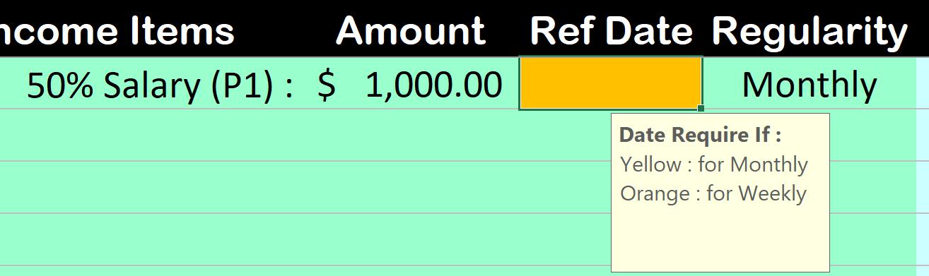 Note that a Reference Date may not always be required. For example – if you are only interested in a Monthly analysis of your income, and you are paid Monthly – then exactly where in the month you get paid doesn’t really matter. At least – not until you change your mind and suddenly decide you want to look at weekly income/expenses. At which point your income sheet needs a date for that Monthly Income.
In this case (see image to the right) – Monthly has been selected as the Regularity, but left the Ref Date cell is left empty. In this case the Ref Date is not actually required for a Monthly Analysis of a Monthly Income; but it would be required for a Weekly Analysis of a Monthly Income – so the cell shows (not so angry) Orange. Easiest solution is to always enter a date if you have it.
5. & 6. Start / Stop Dates.
 It can be seen from Reference Date above (and Regularity below) that a Income setting will propagate forwards and backwards through the Monthly/Weekly planning windows, indefinitely. While this may be ok – you might need to start and/or stop an income from occurring in this way.
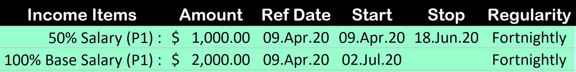
Case in point – the payment on the 9th of April was our first 50% payment, and for the sake of planning you might want to specify an end (Stop) to that and a subsequent beginning (Start) of a return to more “normal” income. The settings shown here accomplish that:
- 50% Salary Starts on 09.Apr.20; Stops on 18.Jun.20; and is Fortnightly based on a Reference Date of 09.Apr.20.
- 100% Salary Starts on 02.Jul.20 (the first pay a fortnight after 18.Jun.20); and does not end; and is Fortnightly based on a Reference Date of 09.Apr.20
![]() There is some basic error checking on Start/Stop Dates. For example, if you enter a Start Date that is after the Stop Date – the cells get angry at you. There’s also a minimum reasonable date in the Settings sheet which can trap accidentally typing in the wrong century and other common date mistakes.
There is some basic error checking on Start/Stop Dates. For example, if you enter a Start Date that is after the Stop Date – the cells get angry at you. There’s also a minimum reasonable date in the Settings sheet which can trap accidentally typing in the wrong century and other common date mistakes.
Note that the Start/Stop Dates are in relation to the Reference Date and Regularity. What this means is that the spreadsheet calculates the date on which something is to be paid using Regularity/Reference Date – then checks the Start/Stop date to see if that is OK. So in the example above – if you entered a Stop Date for the 50% Income line of 17.Jun.20 (one day before the completion of the fortnight) – that payment would not occur in the Planning Sheet because it needed to get to the 18th of June to satisfy a multiple of Fortnights after the Reference Date of 09.Apr.20
7. Regularity.
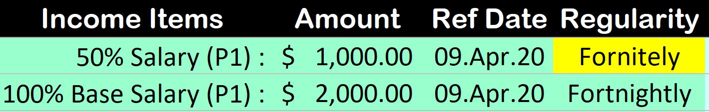 The Regularity selection is used in conjunction with the Reference Date (as well as the Start/Stop Dates) to specify a pattern of income. See Reference Date (above) for more details on how Regularity and Reference Date work together. While a Regularity can be entered (typed), it must match one of the pre-defined selections in the drop-down list. As such it’s best to use the drop down list selection when entering a Regularity.
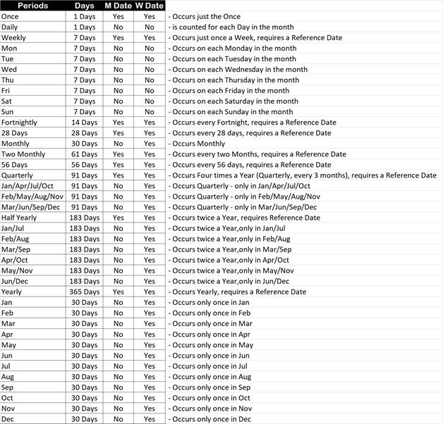 There are many, many Regularity selections. I realise the image of the list here is too small to read, but if you right click (or touch and hold) and open in a new tab you’ll get a full sized image. But quickly …
- Once = Occurs on the Reference Date only, no repeat, limited by Start/Stop Date(s).
- Daily = Every Day, limited by Start/Stop Date(s).
- Weekly (or Mon/Tue/…/Sun) = once a week – either on the day (Mon/Tue…) or on the same day of the week as the Reference Date. As always, limited by Start/Stop Date(s).
- Fortnightly = Every two weeks, on the same day of the week as the Reference Date, limited by Start/Stop Date(s).
- 28 Days = Every four weeks, on the same day of the week as the Reference Date, limited by Start/Stop Date(s).
- 56 Days = Every eight weeks, on the same day of the week as the Reference Date, limited by Start/Stop Date(s).
- Monthly = On the same Date each Month, limited by Start/Stop Date(s).
- Two Monthly = On the same Date every second Month (odd/even), limited by Start/Stop Date(s).
- Quarterly = Every Three Months (four times a year); on the same date in that month as the Reference Date, limited by Start/Stop Date(s).
- Jan/Apr/Jul/Oct or Feb/May/Aug/Nov or Mar/Jun/Sep/Dec = Quarterly, same date as the Reference Date, limited by Start/Stop Date(s).
- Half Yearly = Every Six Months; on the same date in that month as the Reference Date, limited by Start/Stop Date(s).
- Jan/Jul or Feb/Aug or Mar/Sep or Apr/Oct or May/Nov or Jun/Dec = Half yearly, same date in the Month as the Reference Date, limited by Start/Stop Date(s).
- Yearly = Once a Year, on the same Date/Month as the Reference Date, limited by Start/Stop Date(s).
- Jan or Feb or Mar or Apr or May or Jun or Jul or Aug or Sep or Oct or Nov or Dec = Yearly, on the same date as the Reference Date, limited by Start/Stop Date(s).
Note : that there are two columns in the table-image shown here “M.Date” and ‘W.Date” – this is used by the spreadsheet to determine whether a Reference Date is required when a particular Regularity is Selected for the Monthly or Weekly planning. For example – If you select a Monthly income Regularity – you do not require a Reference Date for Monthly Planning – but you do require a Reference Date for Weekly planning. You don’t need to worry about this as the spreadsheet cell colours yellow or orange to indicate (see Reference Date above).
8. Average Income Calculations.
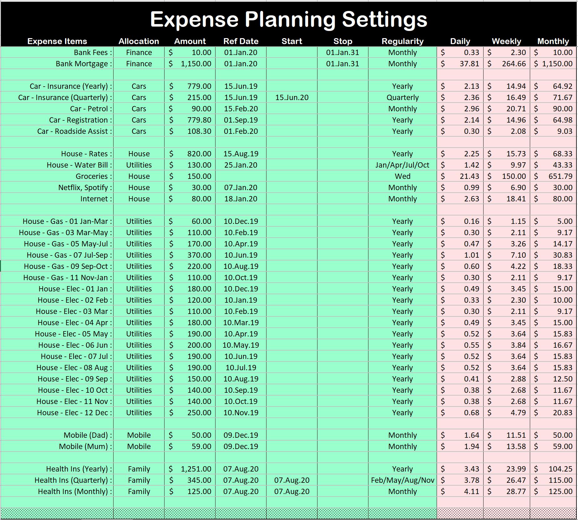
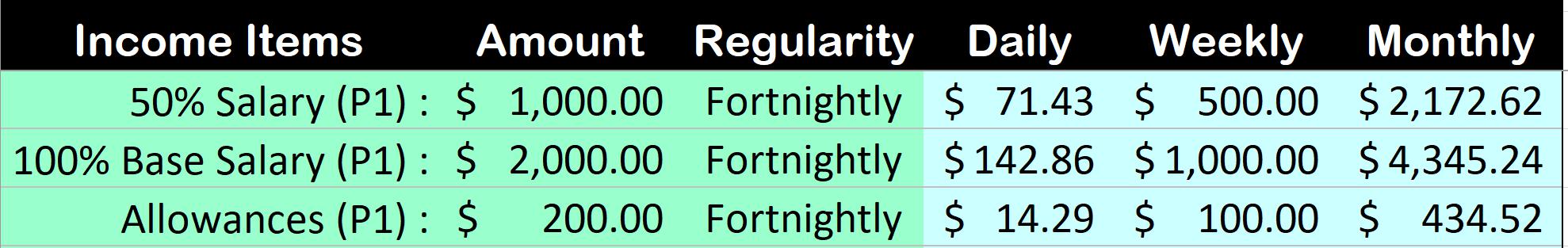 For easy reference – there are three calculated values on the end of each income line. These cells take the Amount and Regularity you specified, and calculates these settings into approximate Daily, Weekly and Monthly values for easy reference (and cross checking). Note that this area is Light Blue – indicating you are in the Income area. The identical area in the Expenses is Light Red (yes, that’s Pink) to remind you that you’re no longer in the Income area.
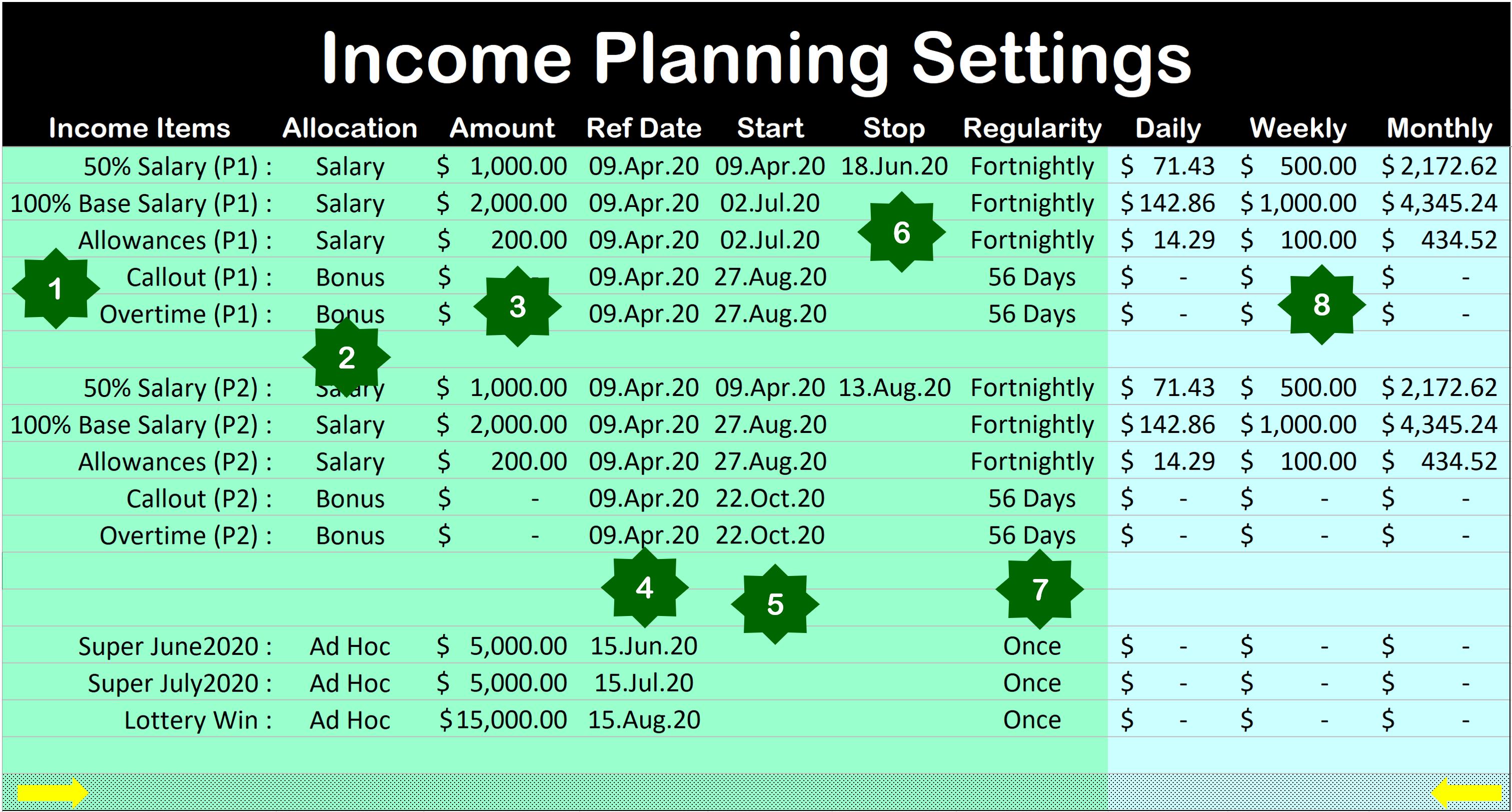
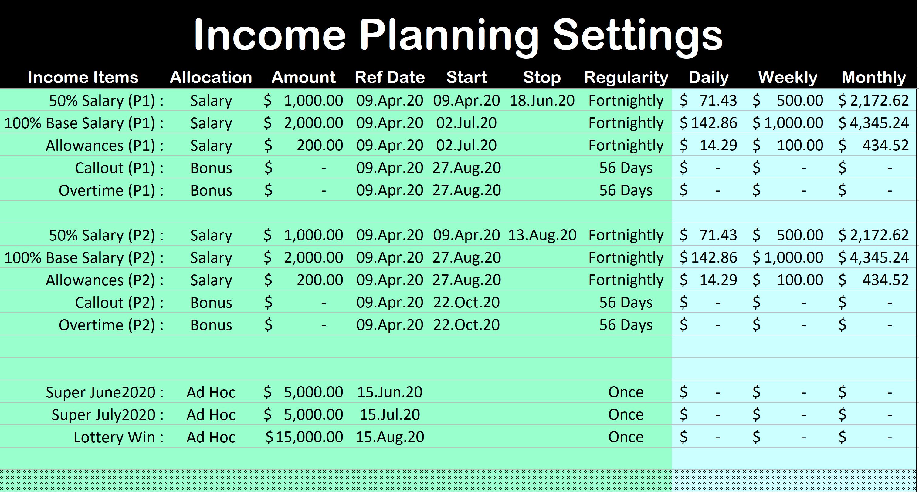
Summing Up – Income Scenario Planning
So from the original image you can see that there are two different scenarios we are considering here:
- Plan 1 : 50% pay from 09.Apr.20 through to the last 50% pay on 18.Jun.20; then 100% pay from 02.Jul.20 and on.
- Plan 2 : 50% pay from 09.Apr.20 – all the way to 13.Aug.20; then 100% pay from 27.Aug.20 on.
- I have boldly allowed for some Allowances to be paid with each fortnightly pay after I return to work!
- Additionally – the ability to add (or not) Super Withdrawals (and the odd Lottery Win!) to the plan(s).
In this way we can build different cases for income – and then select these differently into different planning tabs to see how things are as the COVID-19 impact on the airline industry drags on through the year. Another option would be to remove the Stop Date on the 50% pay and not select in the 100% pay to see what that looks like.
To see how this works out – we first need to review the Expenses tab/worksheet.
The Expenses Sheet
So the Expenses tab is not that much more complicated than Income – you just tend to take more advantage of the potential flexibility of the Reference Date / Regularity Setting and Start/Stop Dates. Since there are no actual changes in these settings between what I previously described on the The Income Sheet – rather than repeating that detail, let’s look at some sample expenses and how they are implemented.
As always – The GREEN areas are designed for your input. The rest of the sheet is locked to ensure you don’t damage the structure/formulas.
Bank Mortgage
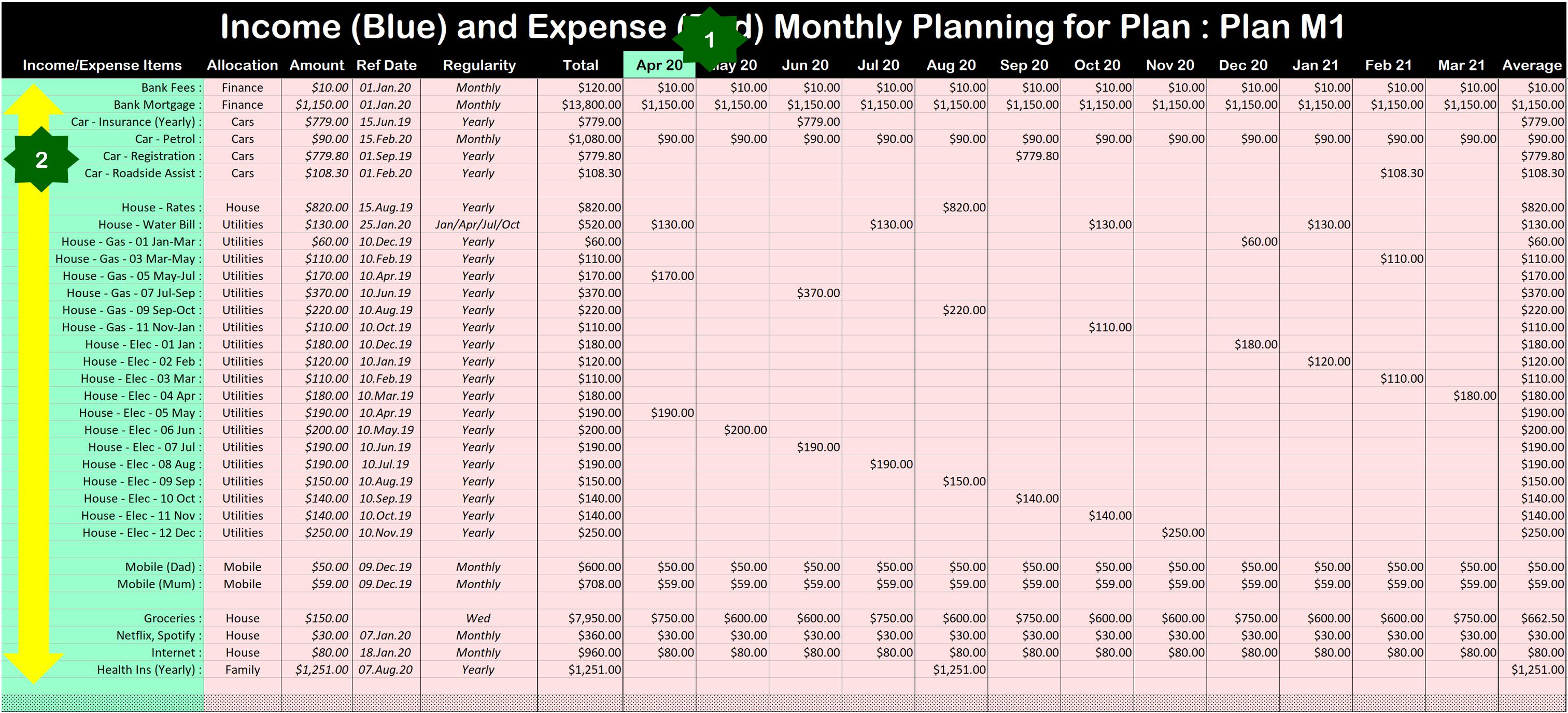
The bank mortgage typically consists of the repayments and potentially some fees. In this case:
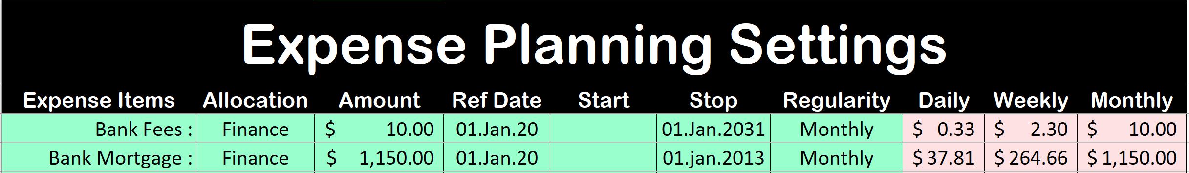
- The Bank Fee is $10; Reference Date 01.Jan.20 with a Monthly Payment. Set to end on 01.Jan.2031
- The Mortgage Payment itself is (presently) $1150; with similar date/regularity parameters.
- As a Monthly payment, the Reference Date is not actually required for a Monthly Analysis – but if you want to look at things weekly – you need to know the date of the month the payment(s) occur so that the sheet can place these in the correct week.
- Note that these are all allocated to Finance, which means potentially these two costs could be grouped for reporting/graphing purposes later.
Car Expenses
Car Expenses introduce a little more variety into the Expense sheet.
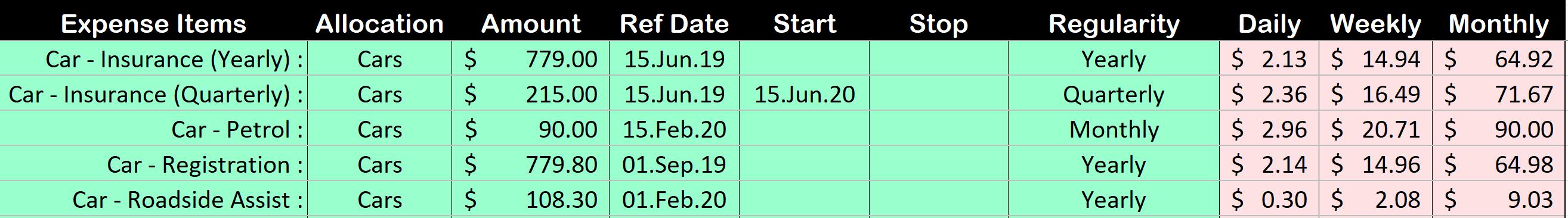
- Car Insurance is Yearly; Reference Date (last paid) on 15.Jun.19.
- Note however that there is a second line for Car Insurance. It turns out that Car Insurance could also be paid Quarterly. So having found out the rate – there is now a second line Car Insurance (Quarterly) with the appropriate cost (obtained from the insurer); same Reference Date of 15.Jun.19 and calculated using a Regularity setting of Quarterly.
- Note that the Car Insurance (Quarterly) line has a Start Date of 15.Jun.20 – you typically can’t go backwards in time and pay your Car Insurance quarterly, you have to change to a quarterly setting at your next payment. By setting the Start Date here as 15.Jun.20 – all we have to do is select this expense into the Planning Window (instead of the Yearly one) and it will apply a quarterly payment on 15.Jun.20 – and every three months after that.
- Worth noting is the increased Daily/Weekly/Monthly cost of the Quarterly vs Yearly payment (the Light-Red-[Pink] area).
- Car Petrol is in here as a Monthly Payment … the Reference Date here allows the spreadsheet to allocate this correctly in the Weekly planning window.
- Registration and Roadside Assist occur Yearly.
House Costs
First some simple House Costs – Rates, Water, Groceries, Netflix/Spotify and Internet.
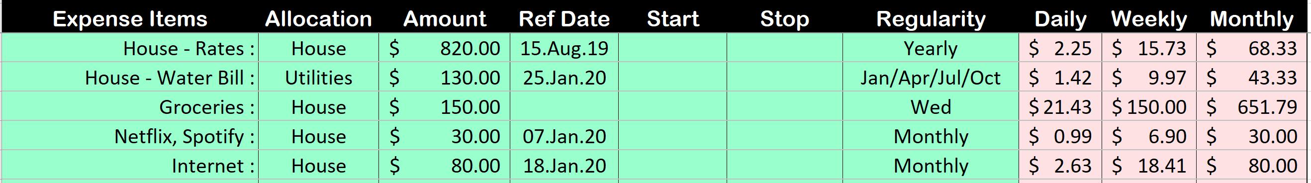
- Rates (Yearly); Netflix/Spotify (Monthly); and Internet (Monthly) are straight forward.
- The Water Bill is approximately the same throughout the year in this house – it’s a Quarterly Payment, due in January – and you can see the Regularity setting chosen here is the Jan/Apr/Jul/Oct quarterly setting (which does not strictly speaking require a Reference Date). With a Reference Date entered, a Regularity setting of “Quarterly” would also have done the job.
- The cost of Groceries is a weekly setting, and for the purposes of planning – happens on a Wednesday.
- The Allocation for Water is as a Utility; the rest are just allocated to House.
House Costs – The Gas Bill
So it turns out my Gas Bill is not simple. While it would be easy to add up the Gas Bill for a year and divide by 6 (it’s paid every TWO MONTHS FOR SOME REASON) – since our Summer gas bill is not much and our Winter gas bill is the GDP of a third world country – I needed some way to plan the costs allowing for this peak/trough situation. Fortunately our gas company has an excellent app that lets us look backwards and see past bills.
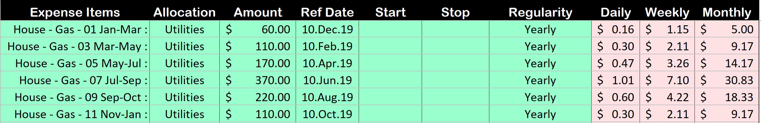
- For the Item Name – I needed something I could easily recognise. So I named them for the months the Gas Bill covered.
- From the first line – you can see that the House Gas Bill for Jan-Mar is actually paid in December, on the 10th. This pattern continues on through the year for the 6 payments (each covering two months) paid the month before. It’s a weird system.
- Even though we pay a Gas Bill every two months – because I have separately entered a year’s worth of bills – all 6 have a Regularity setting of Yearly, so each of them only occur once each year.
- So even though there is a ‘Two Month” selection in Regularity – that doesn’t suit here because I want the payment in June (to cover July/September) to be much more than that in December. (Actually, I don’t want that, I just aren’t given the choice … I live in Melbourne.)
- I’ve also placed the Gas bill in Utility so I can group these together with Water and Electricity.
House Costs – Electricity Bill
The electricity bill similarly has peaks and troughs that I wanted to account for (based on last years consumption).
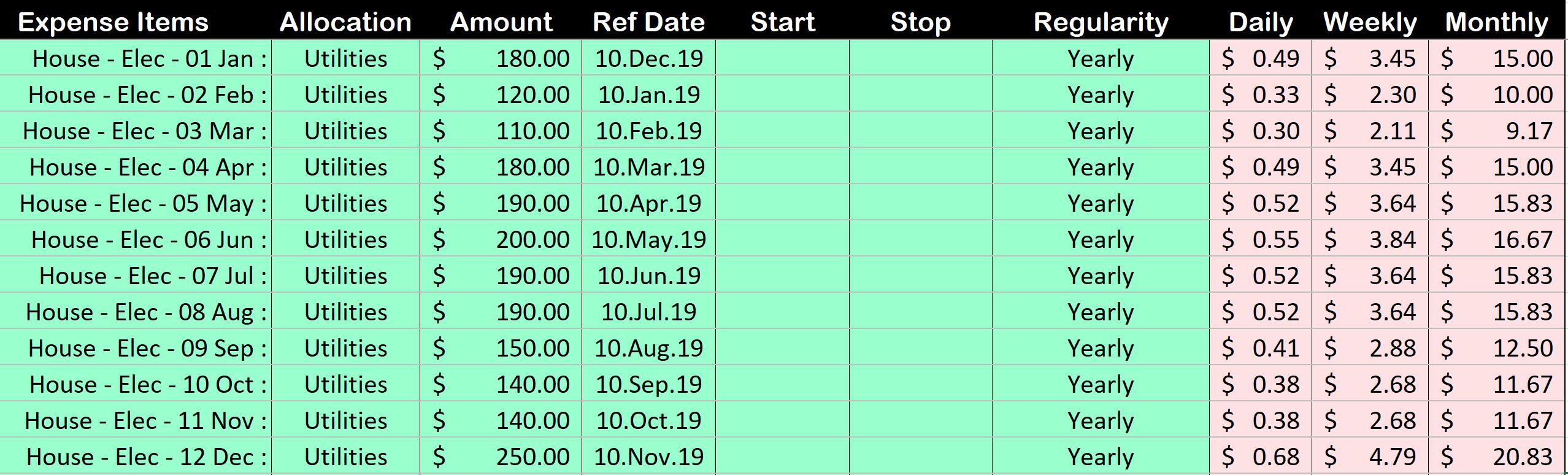
- In this case, our electricity is paid Monthly, on the 10th. To give me maximum flexibility I entered 12 different lines in the sheet, labelling them so I could find and understand them.
- The Amounts vary, all are paid on the 10th of the month before; and once again despite being a Monthly payment – since I have all 12 entered here separately, they are configured with a Regularity setting of Yearly.
Mobile Phone and Health Insurance
While you will have many more expenses (I know I do) let’s finish this off with Mobile Phone and Health Insurance.
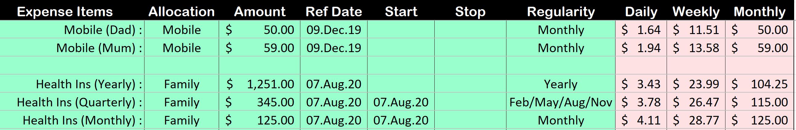
- Mobile Phone is a non-event; Reference Date 09.Dec.19 and paid Monthly.
- There are three potential Health Insurance payments – Yearly, Quarterly and Monthly. Once you get these figures from your Health Insurer, you can enter them in here and see the comparison of costs at the end of the sheet – the more often you pay, the more you pay overall unfortunately.
- Note that the Quarterly and Monthly Payments have a Start Date of 07.Aug.20 – this is the date of the next payment and therefore the next opportunity to convert from Yearly to Quarterly or Monthly.
Summing Up – Expenses Scenario Planning
Just like in the Income Sheet – The expenses sheet can contain not just your current/currently planned expenses – but you can also try out expenses like proposed loans or different versions of significant expenses that can be moved from less often to more often to lessen the burden of particular times of the year. I returned from overseas to Australia in June 2008. As a consequence – practically all our regular bills whether yearly or quarterly fall due in June, making it a particularly bad month to be low on income. Having created possibilities into both Income and Expenses sheets – how try these out is up to you in the Planning Sheet(s).
- The blank lines serve no functional purpose save to separate out your groups of expenses to make the sheet easier to work with.
The Planning Sheets
Since I’ve been referring to the Income and Expense Sheets/Tabs – you’ll no doubt have seen these at the bottom of the Excel workbook. In the SAMPLE download, these are pre-named in accordance with the scenarios I constructed to demonstrate the sheet.
![]()
- Plan M1 and Graph M1 02Jul20 – the 12 Monthly Plan and the 12 Monthly Graph which anticipates a return to work in mid June – or rather first full pay check of 02Jul20.
- Plan M2 and Graph M2 27Aug20 – the 12 Monthly Plan and the 12 Monthly Graph which anticipates a return to work of early August – or rather first full pay check of 27Aug20.
- Plan W1 and Graph W1 02Jul20 – the 16 Week, weekly Plan and Graph anticipating a return to work in mid June.
- Plan W2 and Graph W2 27Aug20 – the 16 Week, weekly Plan and Graph aiming for a first full pay check at the end of August.
Let’s look at a Planning sheet and see how it mixes the Income and Expenses we entered in order to calculate out a budget for us. Note that while the following covers the specifics of the Monthly planning sheets (Plan M1, Graph M1, etc) – the requirements are identical to setup Weekly Planning/Graphs (Plan W1, Graph W1, etc).
Monthly/Weekly Planning Sheet
The Planning Sheets (whether Monthly or Weekly) are in three sections:
- Income – into which you select all the income streams you have created that you want considered in this Plan.
- Expenses – into which you select all the Expenses you want considered into this Plan.
- Totals / Running Balance – which can take initial value (such as money in the bank) and carry that through the difference between your Income and Expenses each Month (or Week in the weekly planning sheets).
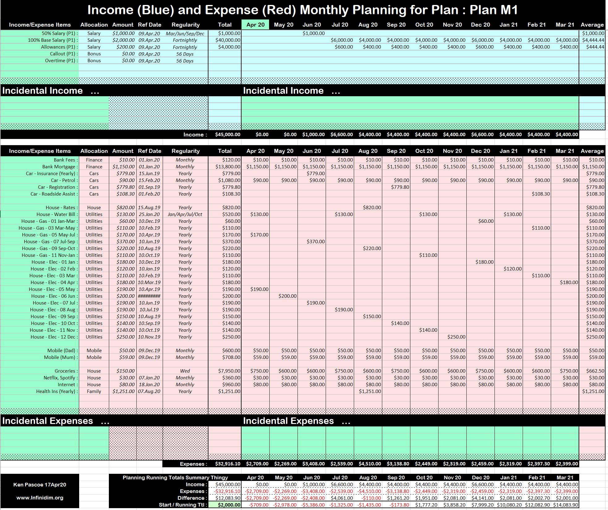
No, you’re not really meant to be able to read this here – but if you did right click (or press and hold) and choose open in another tab you should get a cleared pictures. Lets look over the three sections in detal.
Planning Sheet – Income
The Planning Income requires you to select two items. The first is the starting month of the plan. This cell (shown here with a yellow box) requires you to enter the first day of the month you with to start your 12 month plan for. Since I’m building this in late March/April – I’ve started it in April. But in terms of your regular, repeating (or not) expenses – you can pick any month at all and it will look at that month and the eleven following it, automatically. Having (1) entered a date, you (s) select in all your Income streams, then if necessary (3) add some Ad Hoc expenses. Each time you select an expense – the sheet will calculate out on the right the application of your (Weekly, Fortnightly, Monthly etc) incomes for you.
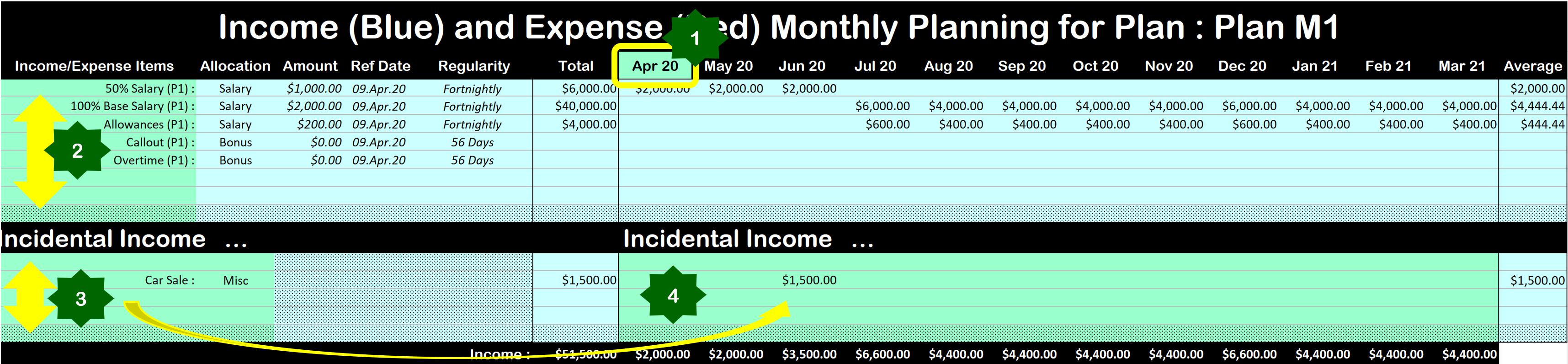
As always – The GREEN areas are designed for your input. The rest of the sheet is locked to ensure you don’t damage the structure/formulas.
1. Date : Enter a date into this cell. The cells to the right will fill with the subsequent months. If they don’t – you’ve probably entered the date incorrectly.
2. 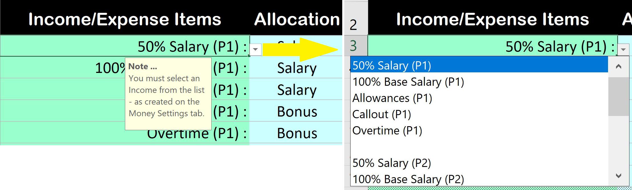 Income Items
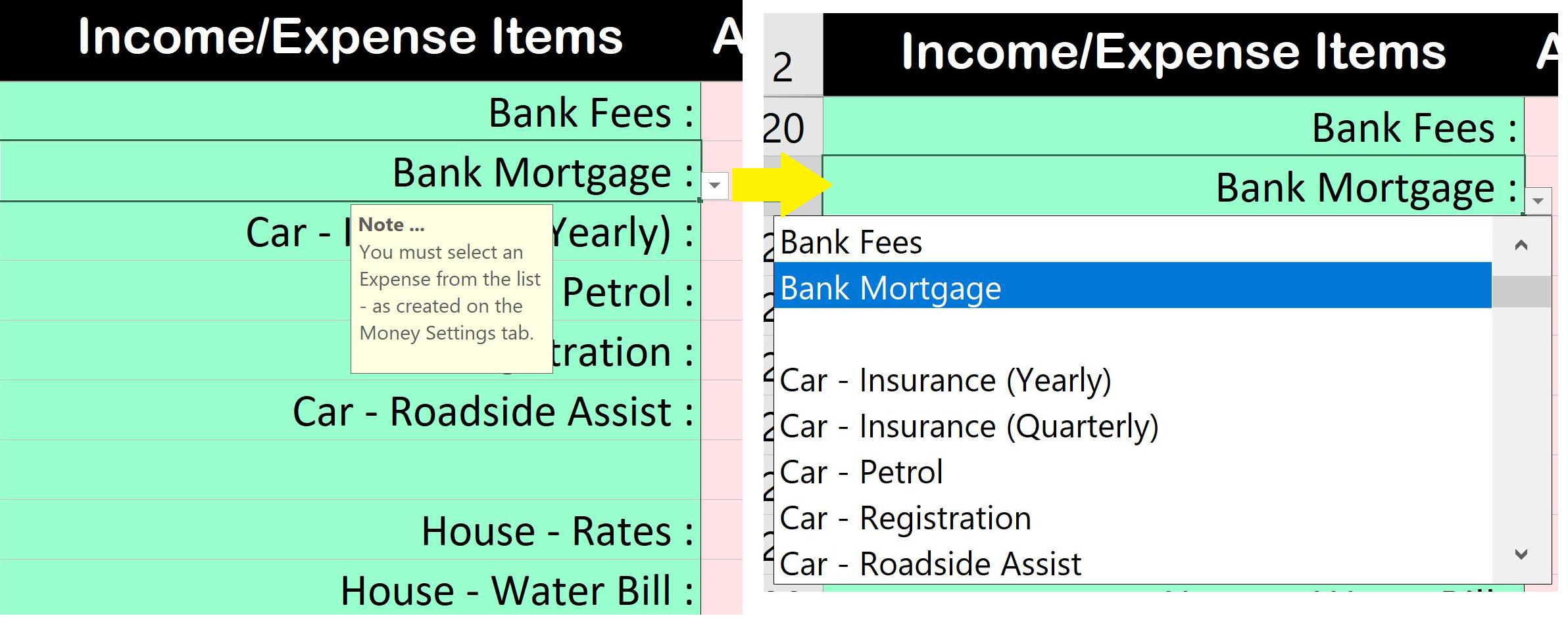
- While you can technically type these in – it’s best to select them from the list. When you click into the cell, a drop down arrow indicates there’s a list to select from. Click on the arrow and the list opens up. Note that owing to a quirk in Excel, the list opens at the very end of the list, so you will have to scroll up to find the top of the list.
- Having selected an Income into a green Income Item cell – scroll across to the right to ensure that the values of Allocation/Amount/Ref Date and Regularity have come in from your Income sheet.
- Then scroll further and see that the Incomes have been laid out correctly in the various months.

You can see from the image above that the 50% Income has made it’s way into April, May, June of 2020. Then from July, you can see the the 100% pay line (three of them) kicking into place. With the return to actual work comes the current estimate of Allowances as well, $200 in each of the fortnightly pays (three of them) in July.
3. 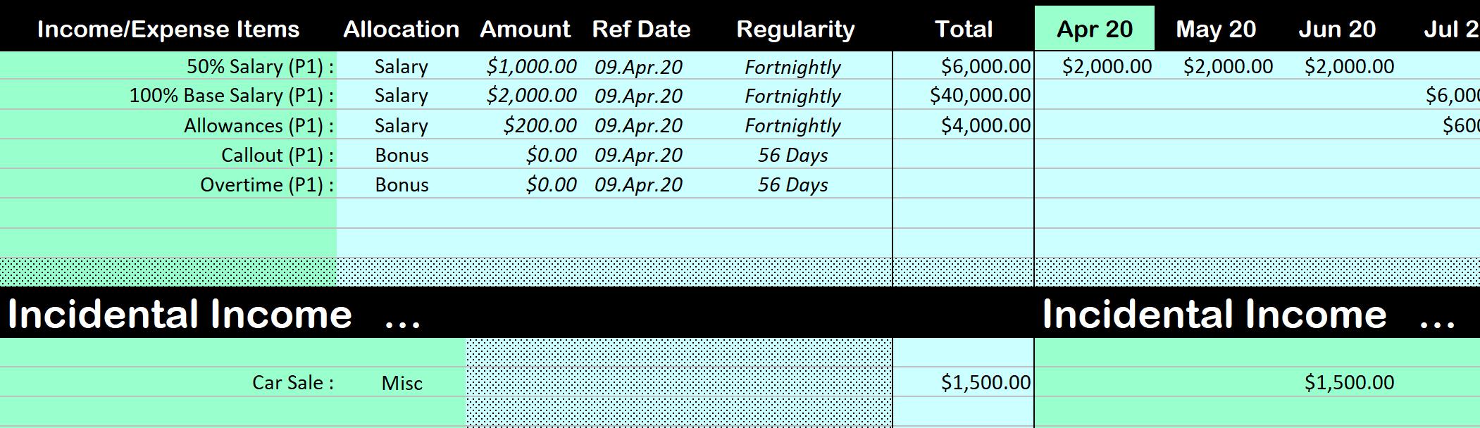 Ad Hoc Income
Ad Hoc income is an area where you can add Income Items that are neither regularly occurring (once off) or items you just want to add into a specific planning scenario. In this case you can see that I’ve added the anticipated sale of a care in June. This is done by (3) giving the Ad Hoc Item a Name (and an Allocation) and then entering the income value under the appropriate month. Note that it’s just as easy (and probably more logical with most Ad Hoc expenses) to enter the sale into the Income sheet, then selected it into the normal Income area of the Planning tab.
Planning Sheet – Expenses
The Expenses area of the Planning sheets is basically the same as income. Select into the Green area the Expense Items (previously created in the Expenses sheet) into the Planning Sheet. Then see the cells across to the right (Allocation, Amount, Ref Date, Regularity) fill in. Further right you can see the Expense Item amounts filling into the cells of the months based on the pattern you created. They Total on the left, and there’s an Average on the right as well.
1.  Date : The date shown here is the same cell as the date you entered for the Income at the top. You only need to enter it once, the spreadsheet is setup with the top two rows as a fixed area as the rest of the cells scroll underneath.
2. Expense Items : Once again – best to select from the list by clicking the little down arrow and choosing from the list. As before – owing to a quirk in Excel for a new selection, the list opens after the last item in the list so you have to scroll up through all the items to get to the one at the top.
Having selected each item – remember to check the expenses are propagating out correctly across the Months.
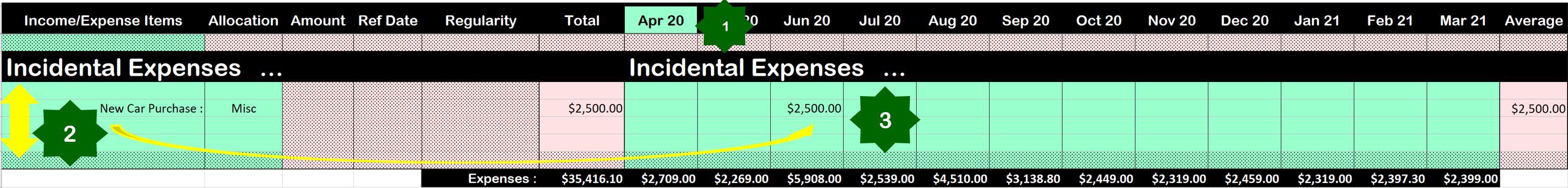
3. Ad Hoc Expenses : Much like Ad-Hoc income – this is where you add (manually) those one-off expenses. Again, logically you could put them into the Expenses sheet and select them into the previous area. You’ll need to enter an Ad Hoc Expense Item Name, an Allocation, and don’t forget to put the actual expense somewhere under the correct Month.
Planning Sheet – Summary
At the bottom of the Planning Sheet(s) is the summary area. This section produces a summary of Income vs Outgo (Expenses) for each month, as well as a total. There is also a line to carry forward the result of (Income – Minus – Expenses), which is carried on from month to month. There is a green cell to the left of the Running Total called the Start – enter an amount (positive or negative) in this cell as your starting figure and the Running Total will start with this figure and carry it through the months,
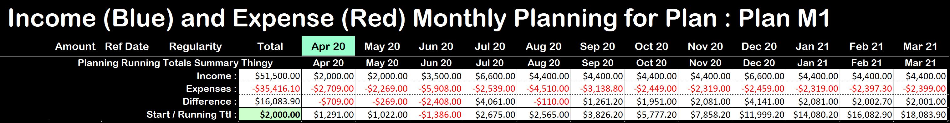
This summary is one of the two purposes behind all this work. To see how much each Month/Week is costing you vs your income – and to see how this carries out over time. But while Numbers are great – a visual representation is always useful, so lets look at the sample graph I built.
Note that while the following covers the specifics of the Monthly planning sheets (Plan M1, Graph M1, etc) – the requirements are identical to setup Weekly Planning/Graphs (Plan W1, Graph W1, etc).
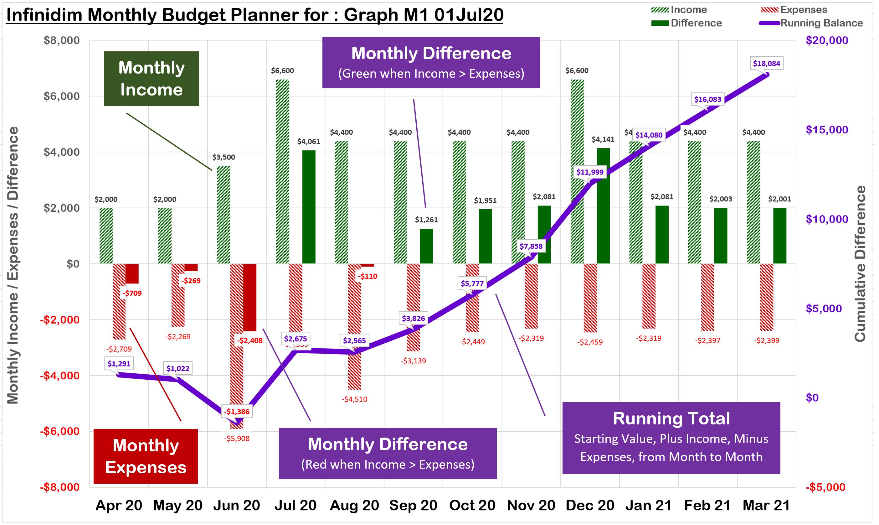
The Graph Sheets
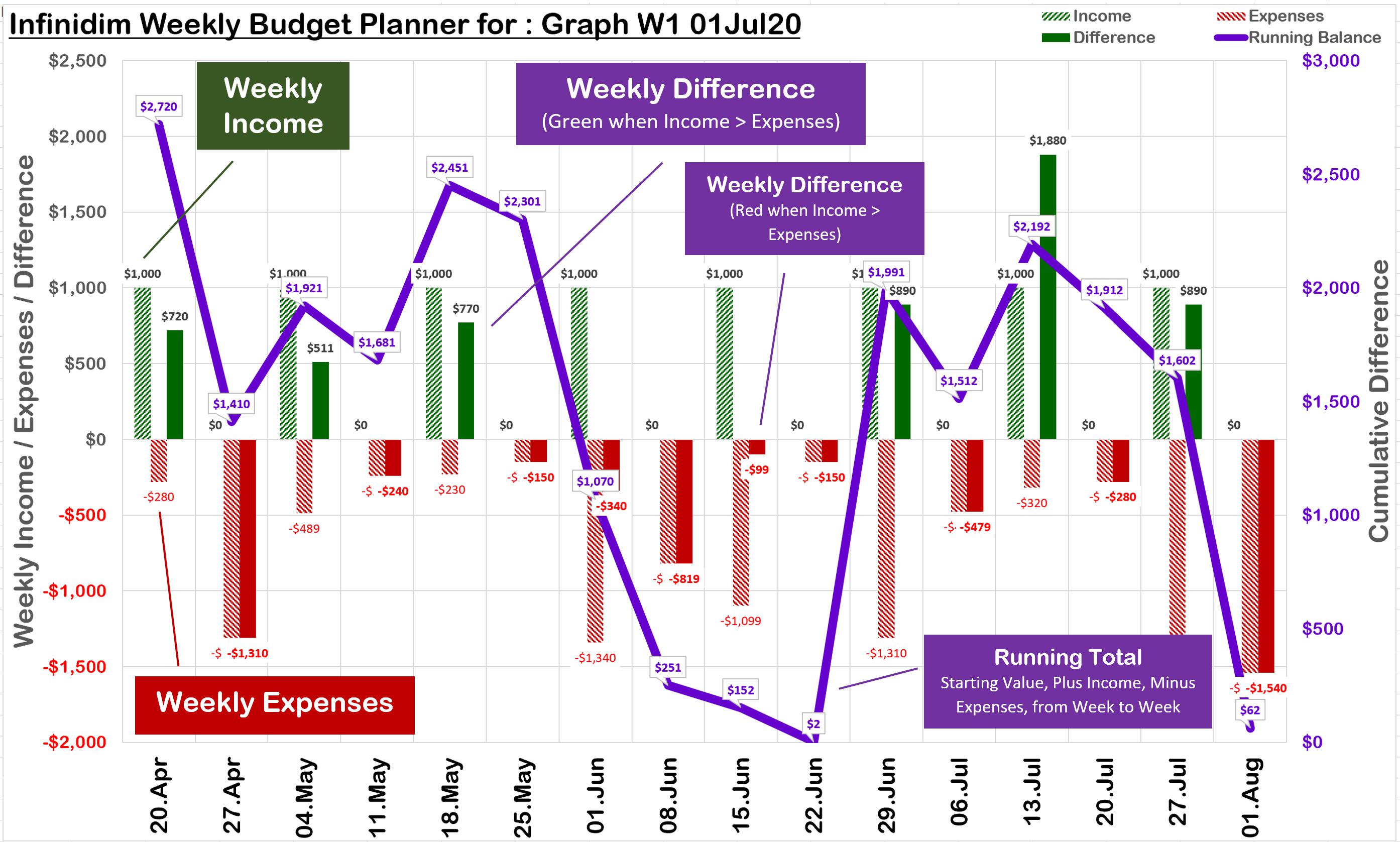
I’ve only done one type of graph, but I’ve put a bit of work into it to make it as useful (and clear) as I can.
- The basic horizontal axis has the 12 Months of the Planning Window from your Planning sheet.
- The left vertical axis represents the $ values of your Monthly Income, Expenses and Difference (Difference = Income – Expenses)
- The striped green bars are the Total Income for each Month.
- The striped red bars are the Total Expenses for each Month.
- The solid Green (good) or Red (not so good) bars are the Difference calculation (Green meaning income exceeded expenses for that month; Red means …)
- Over top of this is the Purple Line that is the Running Total – starting with the value you specified in the sheet (or zero if you did not specify one). Note that the axis for this purple line is actually on the RHS. In the example given, the initial Purple Line value is +$1291 (pre-April starting value of $2000, reduced by the bad Month of April with a Difference of -$709). So when looking at the purple line – look to the right for the scale.
Weekly Budget – Planning & Graph
At this point’ we’ve covered the Income Sheet, the Expenses Sheet, one Monthly Planing Sheet, and the associated Monthly Graph. The Weekly Planning and Graphing sheets are basically identical as you can see here, and draw from the exact same Incomes and Expenses you specified in the Income and Expenses sheets:
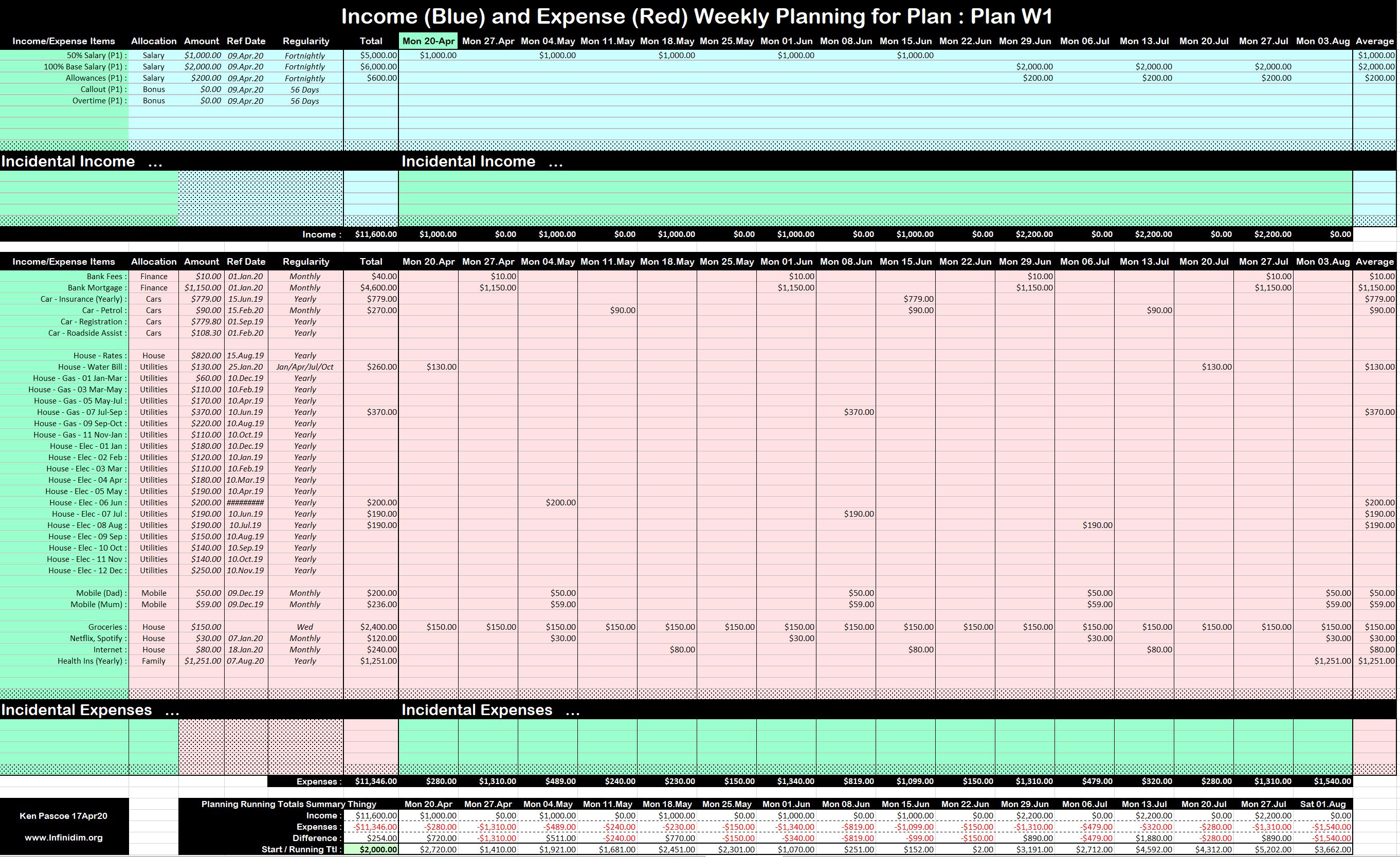
- You structure is essentially identical, except that it’s Weekly Planning Window – and it runs for 15 weeks (4×28 Day Rosters; or 2×56 Day Rosters).
- Specify the Start Date for your Planning Window.
- Enter (select) your Income(s) and Expenses in the Green Areas. As you enter each one, check the Allocation, Amount, Ref Date and Regularity come across – and check the values show under the appropriate weeks.
- Incidental Income and Incidental Expenses also work the same – don’t forget to enter the amount under the correct week.
- Totals and Running Totals work the same.
Onto the Weekly Graph. As you’d expect – no surprises here, it looks like the Monthly Graph … except Weekly.
Payslip / Roster Period Worksheet
A late development is the requirement for crew to nominate up to 14 days in a Roster Period as Leave (rather than Leave Without Pay) in order to convert up to 50% of our stand-down roster into something that generates some income while using available leave. I have been using the following sheet to forecast what I’m likely to get in each of the 14 day payslips,
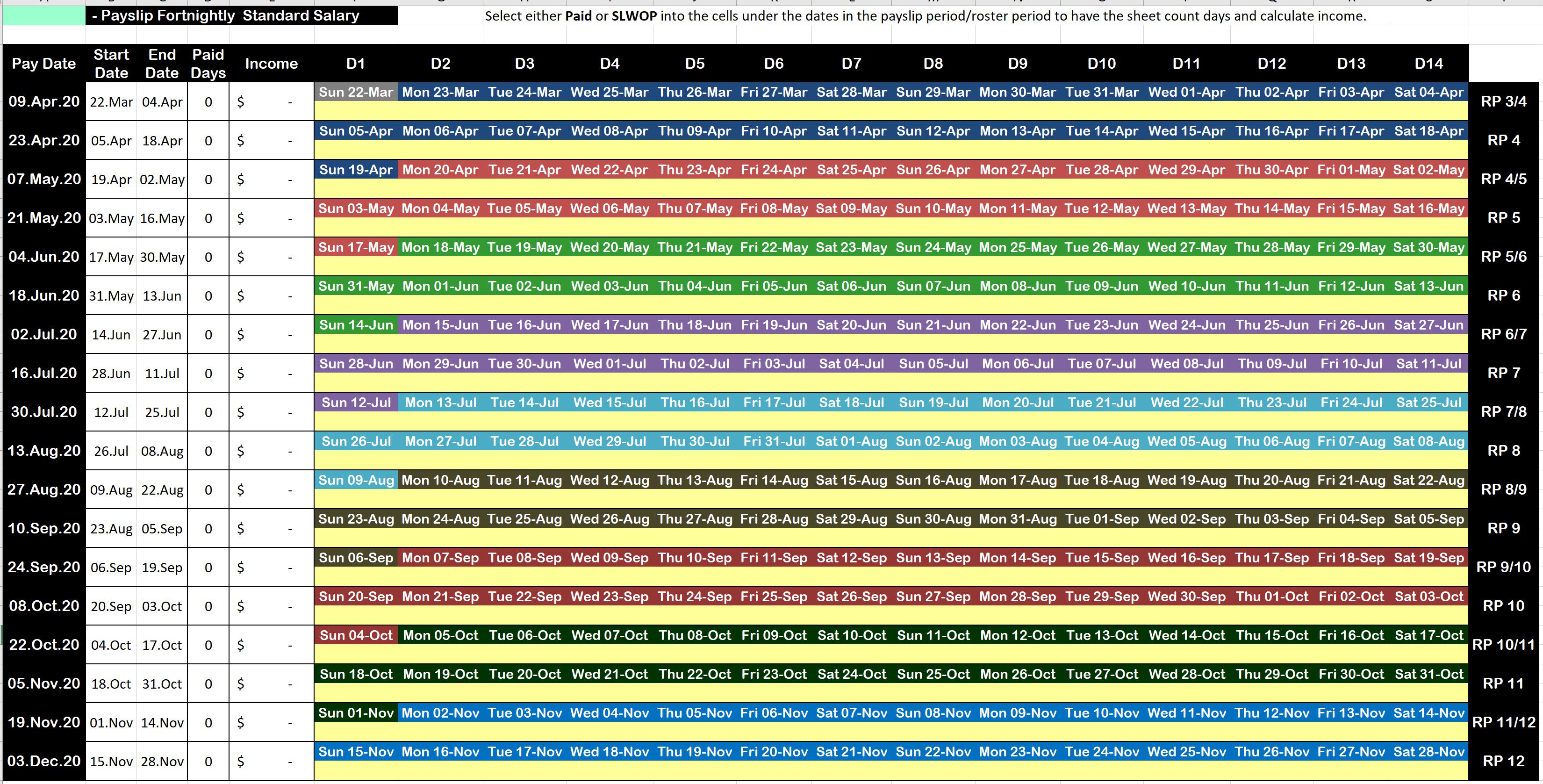
- Enter your Gross (or if you can work it out, Net) Standard 14 day salary from your most recent Payslip.
- Enter/Select either “Paid” or “SLWOP” into the rows of empty (yellow) cells under the dates of the Payslip 14 day row. (Note only the “Paid” entries matter.)
- The sheet will add up the “Paid” dates; and multiple this out to calculate an approximate income.
Some Excel Tips
You’re going to have to know how to do the following in order to really use the spreadsheet. If you aren’t sure – watch the training video to see how.
- Many cells have pre-built drop down lists. When you click into a cell (such as a Allocations) you will see a small drop down list box on the right – this allows you to select from a pre-built list (if it exists)
- Anything cells that are Green means it’s an area that you are allowed to make input into. To protect the formulas – the rest of the sheet is protected against erroneous input. If you want access to build your own version – the password is … empty
- If a Green cell suddenly turns (bright/strong) Yellow – that indicates that an entry is required in that cell to complete the line correctly. Orange indicates that a Ref Date would be required if this Income/Expense is to be used on a Weekly Plan.
- Entering Dates needs a little caution. Unfortunately the inclusion of a date picker control could break the sheet on different versions of Excel (even just across Windows) so I’ve left it to native Excel. I always enter dates as “dd MMM (yy)” (spaces between) this means – two digit date, space, three letter year and if I need the year to be other than this one – space, a two digit date. So … “12 Mar” -> 12.Mar.20 … or … 12 Mar 19 -> 12.Mar.19. In the end after you have entered your date – if it looks wrong or the background turns yellow, try again. Note that depending on your Windows settings, the resulting date might look different – 15.Jul.20 (mine) or yours – 15-Jul-20 or 07/15/20 (US), etc.
- Do not use the last Row of any section in a Sheet. You’ll notice the last row has dots all over it anyway to tell you not to use it. Point of fact – it’s better not to use the second last row either – leave it empty so you can copy it to make more room. Speaking of that …
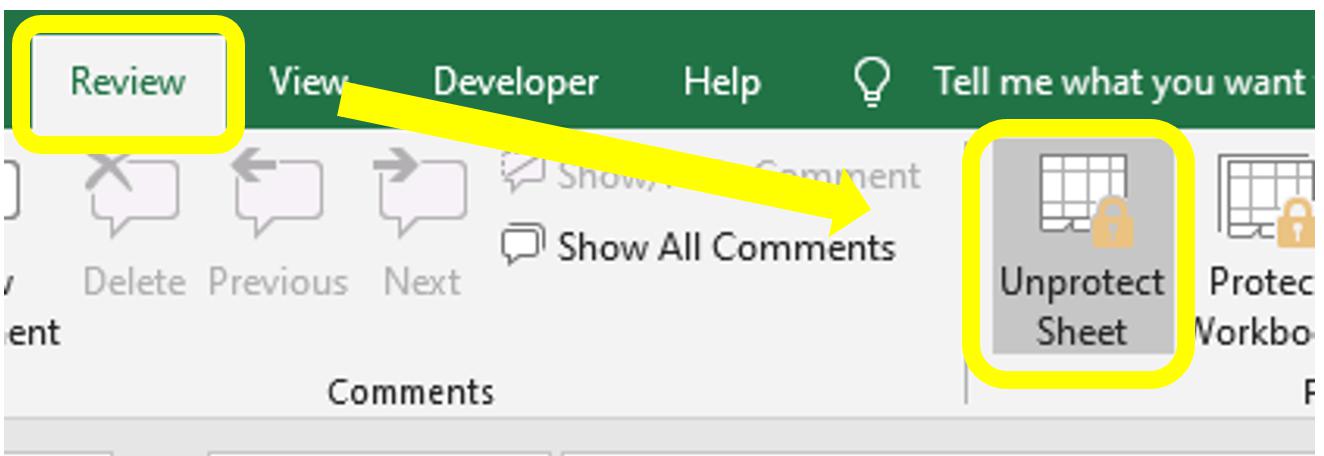
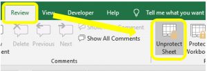 You might need to insert rows into the sheet. To do this you will first need to Unprotect the sheet. All the sheets are protected from making change to other than the Green areas to stop you from damaging the structure or formulas. Click on Review up to top and then look for the Unprotect Sheet button in the ribbon. Click Unprotect Sheet and the sheet is now ready for you to damage.
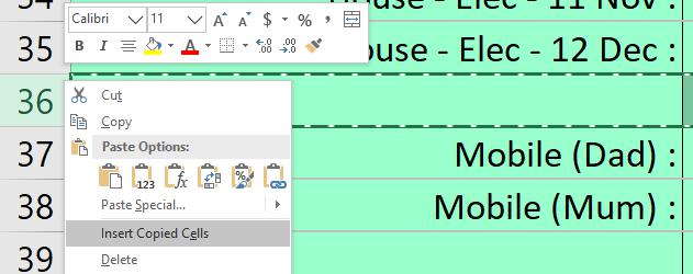
 Now right-click on the row number on the far LHS of the sheet, against an empty row. You must choose an empty row – and it must not be the row at the bottom of a section of the sheet (these are green, but marked with little dots to tell you not to go there).So – right click beside an empty row, and choose Copy.
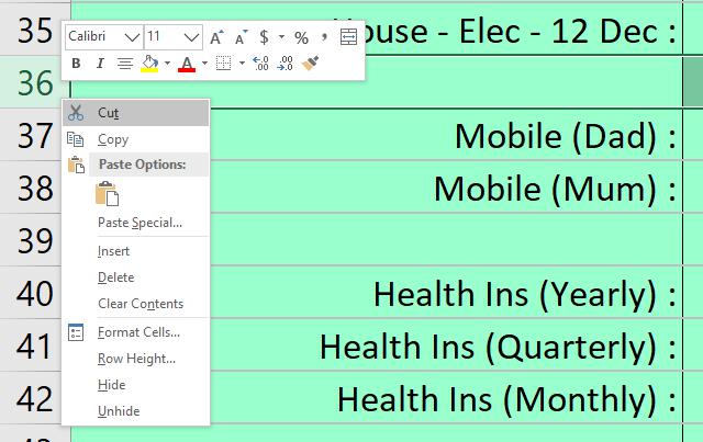
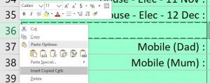 Having copied the entire empty row (and you will now see all that row being highlighted with dashes circling the boundary of the copy area). Now right click against another row (or the same one) in the same section where you want to insert a copy of that blank row from before. This time, choose Insert Copied Cells – and a new blank row will appear.
- Note that you can right-click-hold-and-drag down across a few empty rows, copy them, and insert a copy of these multiple blank rows into your sheet.
Training Videos
I made some training videos to explain how to use the sheet. For this go round, I decided to keep them as short as possible and address individual topics so you can pick and choose – then practice.
Ken.
If you find my content useful and are in a position to do so – I would appreciate a contribution to my PayPal account (ken.pascoe@gmail.com) – If you use the Friends and Family feature in PayPal it reduces the charges to the transfer. Please note that when sending money in this way you are removing any form of purchase protection, which is not relevant to a contribution of this type anyway.